Chapter 8 Hypothesis Testing
Learning Outcome
Perform hypotheses testing involving one population mean, one population proportion, and one population standard deviations/variance.
This chapter introduces the statistical method of hypothesis testing to test a given claim about a population parameter, such as proportion, mean, standard deviation, or variance. This method combines the concepts covered in the previous chapters, including sampling distribution, standard error, critical scores, and probability theory.
8.1 Hypothesis Testing
In statistics, a hypothesis is a claim or statement about a property of a population.
A hypothesis test (or test of significance) is a procedure for testing a claim about a property of a population.
The null hypothesis (\(H_0\)) is a statement that the value of a population parameter (such as proportion, mean, or standard deviation) is equal to some claimed value.
The alternative hypothesis (\(H_A\)) is a statement that the parameter has a value that somehow differs from the null hypothesis.
Purpose of a Hypothesis Test
The purpose of a hypothesis test is to determine how plausible the null hypothesis is. At the start of a hypothesis test, we assume that the null hypothesis is true. Then we look at the evidence, which comes from data that have been collected. If the data strongly indicate that the null hypothesis is false, we abandon our assumption that it is true and believe the alternate hypothesis instead. This is referred to as rejecting the null hypothesis.
The evidence comes in the form of a test statistic. When the difference between the test statistic (such as, \(z\) or \(t\) scores) and the value in the null hypothesis is sufficiently large, we reject the null hypothesis.
\[ \fbox{Assume the null hypothesis is true} \xrightarrow{} \fbox{consider the evidence} \xrightarrow{} \fbox{decide whether to accept or reject the null hypothesis} \]
Example:
Probability of getting head from a single toss of coin, \(p = 0.5\).
Therefore, expected value of the number of heads from \(20\) tosses = \(10\).
Suppose, on your first trial, you have tossed a coin \(20\) times and seen \(15\) heads, \(\hat p = 0.75\).
On your second trial, you have tossed a coin \(20\) times again and seen \(12\) heads, \(\hat p = 0.60\).
Is the coin fair, or is it biased towards heads?
Null and Alternative Hypotheses
Null hypothesis \((H_0)\): states that any deviation from what was expected is due to chance error (i.e. the coin is fair).
Alternative hypothesis \((H_A)\): asserts that the observed deviation is too large to be explained by chance alone (i.e. the coin is biased towards heads).
\[ H_0: p = 0.5 \\ H_A: p > 0.5 \]
Now, what is the probability of \(p \ge 0.75?\) What is the probability of \(p \ge 0.60?\)
From normal approximation of the sampling distribution of \(\hat p\),
\[ \begin{align} p &= 0.5 \\ se &= \sqrt{(0.5)(0.5)/20} = 0.112 \\ z_1 &= (0.75 - 0.50)/0.112 = 2.236 \\ \\ z_2 &= (0.60 - 0.50)/0.112 = 0.893 \\ \\ \text {p-value} &= \begin{cases} P(z\ge 2.236) &= 0.0127 \\ P(z\ge 0.893) &= 0.1860 \end{cases} \end{align} \]
We see that the farther the test statistic is from the values specified by \(H_0\), the less likely the difference is due to chance - and the less plausible becomes. The question then is: How big should the difference be before we reject \(H_0\)?
To answer this question, we need methods that enable us to calculate just how plausible \(H_0\) is. Hypothesis tests provide these methods taking into account things such as the size of the sample and the amount of spread in the distribution.
Interpretation of \(\text{p-value}\)
A \(\text{p-value}\) is the probability of obtaining the observed effect (or larger) under a “null hypothesis”. Thus, a \(\text{p-value}\) that is very small indicates that the observed effect is very unlikely to have arisen purely by chance, and therefore provides evidence against the null hypothesis.
It has been common practice to interpret a \(\text{p-value}\) by examining whether it is smaller than particular threshold values or “significance level”. In particular, \(\text{p-values}\) less than \(5\%\) are often reported as “statistically significant”, and interpreted as being small enough to justify rejection of the null hypothesis. By definition, the significance level \(\alpha\) is the probability of mistakenly rejecting the null hypothesis when it is true.
\[\textbf {Significance level } \alpha = P \textbf { (rejecting } H_0 \textbf { when } H_0 \textbf { is true)} \]
In common practice, \(\alpha\) is set at \(10\%, 5\%\) or \(1\%\).
In the coin toss example:
p-value = \(1.27\%\) which is less than the \(5\%\) significance level.
Therefore, the result is statistically significant.
Conclusion: The coin is biased towards heads.
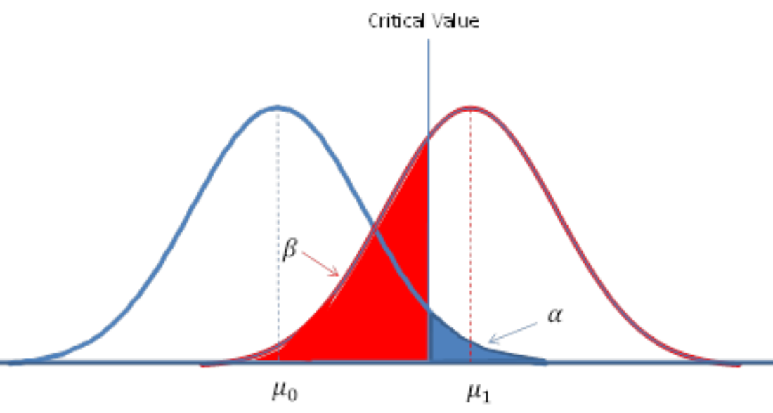
Type I and Type II Errors
When testing a null hypothesis, sometimes the test comes to a wrong conclusion by rejecting it or failing to reject it. There are two kinds of errors: type I and type II errors.
- \(\textbf {Type I error} :\) The error of rejecting the null hypothesis when it is actually true.
\(\alpha = P (\textbf{type I error}) = P (\text{rejecting } H_0 \text{ when } H_0 \text{ is true } )\)
The probability of \(\text {Type I}\) can be minimized by choosing a smaller \(\alpha\).
- \(\textbf {Type II error} :\) The error of failing to reject the null hypothesis when it is actually false.
\(\beta = P (\textbf{type II error}) = P (\text{failing to reject } H_0 \text{ when } H_0 \text{ is false} )\)
The probability of \(\text {Type II}\) can be minimized by choosing a larger sample size \(n\).
In general, a \(\text{Type I}\) error is more serious than a \(\text{Type II}\) error. This is because a \(\text{Type I}\) error results in a false conclusion, while a \(\text{Type II}\) error results only in no conclusion. Ideally, we would like to minimize the probability of both errors. Unfortunately, with a fixed sample size, decreasing the probability of one type increases the probability of the other.
Hypothesis tests are often designed so that the probability of a \(\text{Type I}\) error will be acceptably small, often \(0.05\) or \(0.01\). This value is called the significance level of the test.
Significance Level
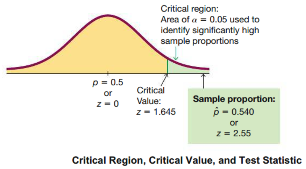
Notice that if \(H_0\) is actually true, but \(\hat p\) falls in the critical region, then a \(\text{Type I}\) Error occurs. We begin a hypothesis test by setting the probability of a \(\text{Type I}\) Error. This value is called the significance level and is denoted by \(\alpha\). The area of critical region is equal to \(\alpha\). The choice of \(\alpha\) is determined by how strong we require the evidence against \(H_0\) to be in order to reject it. The smaller the value of \(\alpha\), the stronger we require the evidence to be.
Critical Value Method
In a hypothesis test, the critical value(s) separates the critical region (where we reject the null hypothesis) from the values of the test statistic that do not lead to rejection of the null hypothesis.
With the critical value method of testing hypothesis, we make a decision by comparing the test statistic to the critical value(s).
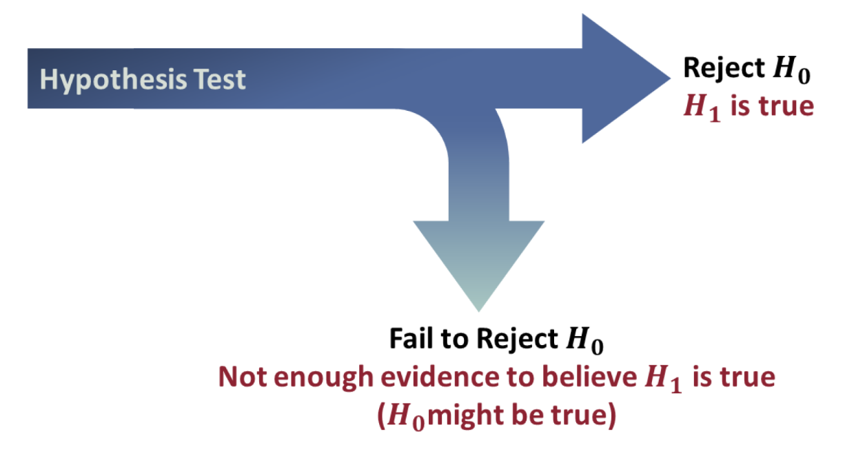
Stating the Conclusion in a Hypothesis Test
If the null hypothesis is rejected, the conclusion of the hypothesis test is straightforward: We conclude that the alternate hypothesis, \(H_0\), is true.
If the null hypothesis is not rejected, we say that there is not enough evidence to conclude that the alternate hypothesis, \(H_a\), is true. This is not saying the null hypothesis is true. What we are saying is that the null hypothesis might be true.
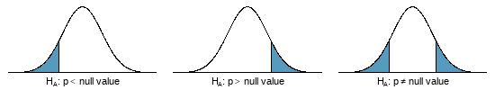
One-sided and two-sided tests
If the researchers are only interested in showing an increase or a decrease, but not both, use a one-sided test. If the researchers would be interested in any difference from the null value - an increase or decrease - then the test should be two-sided.
After observing data, it is tempting to turn a two-sided test into a one-sided test. Hypotheses must be set up before observing the data. If they are not, the test must be two-sided.
Steps of a Formal Test of Hypothesis
Follow these seven steps when carrying out a hypothesis test.
- State the name of the test being used.
- Verify conditions to ensure the standard error estimate is reasonable and the
point estimate follows the appropriate distribution and is unbiased.
- Write the hypotheses and set them up in mathematical notation.
- Identify the significance level \(\alpha\).
- Calculate the test statistics (e.g. \(z\)), using an appropriate point estimate of the paramater of interest and its standard error.
\[\text{test statistics} = \frac{\text{point estimate - null value}}{\text{SE of estimate}}\]
- Find the \(\text{p-value}\), compare it to \(\alpha\), and state whether to reject or not reject the null hypothesis.
- Write your conclusion in context.
8.2 Power of a Hypothesis Test (Optional)
The power of a hypothesis test is the probability \(1-\beta\) of rejecting a false null hypothesis. The value of the power is computed by using a particular significance level \(\alpha\) and a particular value of the population parameter that is an alternative to the value of assumed true in the null hypothesis.
In practice, statistical studies are commonly designed with a statistical power of at least \(80%\).
Post-hoc Power Calculation for One Study Group vs. Population
Suppose,
\[ H_0 : p = P_0 \\ H_A : p \ne P_0 \\ \] \[ \begin{align} P_0 &= \text{proportion of population} \\ P_1 &= \text{proportion observed from the data (an alternative population)} \\ N &= \text{sample size} \\ \alpha &= \text{probability of type I error} \\ \beta &= \text{probability of type II error} \\ z &= \text{critical z score for a given } \alpha \text { or } \beta \end{align} \]
Suppose, \(P_1\) is an alternative to the value assumed in \(H_0\).
Under \(H_0\),
\[ P'_0 = P_0 + z_{1-\alpha/2} \cdot \sqrt{\dfrac{P_0Q_0}{N}} \]
Under \(H_A\),
\[ \therefore z_{\beta} = \dfrac{P'_0 - P_1}{\sqrt{\dfrac{P_1Q_1}{N}}} = \dfrac{\Bigg( P_0 + z_{1-\alpha/2} \cdot \sqrt{\dfrac{P_0Q_0}{N}} \Bigg) - P_1}{\sqrt{\dfrac{P_1Q_1}{N}}} \\ \\ P(\textbf{Type II error}) = \beta = \Phi \left \{ \dfrac{\Bigg( P_0 + z_{1-\alpha/2} \cdot \sqrt{\dfrac{P_0Q_0}{N}} \Bigg) - P_1}{\sqrt{\dfrac{P_1Q_1}{N}}} \right \} \\ \]
\[ \begin{align} \text{where,} \\ Q_0 &= 1 - P_0 \\ Q_1 &= 1 - P_1 \\ \Phi &= \text{cumulative normal distribution function} \end{align} \]
Example: Calculate statistical power for various alternative hypotheses.
\[ Suppose, \begin{cases} H_0: p = 0.5 \\ H_A: p \ne 0.5 \\ P(\text{type I error}) = \alpha = 0.05 \\ \text{Critical z score, } z_{1 - \alpha/2} = 1.96 \\ N = 14 \\ \end{cases} \]
\[ \begin{array}{r|r|r} P_1 & \Phi(z_{\beta}) = \beta & 1-\beta \\ \hline 0.6 & \Phi(1.2367) = 0.8919 & 0.1081 \\ 0.7 & \Phi(0.5055) = 0.6934 & 0.3066 \\ 0.8 & \Phi(-0.3562) = 0.3608 & 0.6392 \\ 0.9 & \Phi(-1.7222) = 0.0425 & 0.9575 \\ \hline \end{array} \]
Example: Sample size calculation to achieve power (when \(P_0\) and \(P_1\) are known)
\[ \begin{align} z_{\beta} = \Phi^{-1}(\beta) &= \dfrac{\Bigg( P_0 + z_{1-\alpha/2} \cdot \sqrt{\dfrac{P_0Q_0}{N}} \Bigg) - P_1}{\sqrt{\dfrac{P_1Q_1}{N}}} \\ \\ z_{1-\alpha/2} &= 1.96 \\ 1- \beta &= 0.8 \\ \\ \Phi^{-1}(0.2) = -0.84 &= \dfrac{\Bigg( 0.5 + 1.96 \cdot \sqrt{\dfrac{(0.5) (0.5)}{N}} \Bigg) - 0.9}{\sqrt{\dfrac{(0.9)(0.1)}{N}}} \\ \implies N &= \Bigg( \dfrac{1.96\sqrt{0.25} + 0.84\sqrt{0.09}}{0.4} \Bigg)^2 \\ &\approx 10 \end{align} \]
Example: Sample size calculation to achieve power (when \(P_0\) and \(P_1\) are unknown)
\[ N = \Bigg( \dfrac{z_{1-\alpha/2} + z_{1-\beta}}{ES} \Bigg)^2 \\ \] where,
\[ \text{effect size, } ES = \dfrac{|P_1-P_0|}{\sqrt{P_0Q_0}} \]
Statistical power and design of experiment: When designing an experiment, it is essential to determine the minimize sample size that would be needed to detect an acceptable difference between the true value of the population parameter and what is observed from the data. A \(5\%\) significance level \((\alpha)\) and a statistical power of at least \(80\%\) are common requirements for determining that a hypothesis test is effective.
8.3 Inference for a Single Proportion
Conduct a formal hypothesis test of a claim about a population proportion \(p\).
Requirements:
- The sample observations are simple random sample.
- The trials are independent with two possible outcomes.
- The sampling distribution for \(\hat p\), taken from a sample of size \(n\) from a population with a true proportion \(p\), is nearly normal when the sample observations are independent and we expect to see at least \(10\) successes and \(10\) failures in our sample, i.e. \(np \ge 10\) and \(n(1-p) \ge 10\). This is called the success-failure condition. If the conditions are met, then the sampling distribution of \(\hat p\) is nearly normal with mean \(\mu_{\hat p} = p\) and standard deviation \(\sigma_{\hat p} = \sqrt {\dfrac{p(1-p)}{n}}\).
\[ \begin{cases} n = \text {sample size } \\ \hat p = \dfrac{x}{n} \text { (sample proportion) } \\ p = \text {population proportion } \\ q = 1 - p \\ \end{cases} \]
Test Statistic for Testing a Claim About a Proportion
\[ z = \dfrac{\hat p - p}{\sqrt {\dfrac{pq}{n}} } \]
Example:
The DMV claims that \(80\%\) of all drivers pass the driving test. In a survey of \(90\) teens, only \(61\) passed. Is there evidence that teen pass rates are significantly below \(80\%?\)
Let’s say, \(p\) is the true population proportion.
\[ \begin{align} \text {One-tailed test} &:\\ H_0&: p = 0.80 \\ H_A&: p < 0.80 \end{align} \]
Verify success-failure condition:
\[
\begin{align}
np \ge 10 \rightarrow 90 \times 0.80 \ge 10 \\
n(1-p) \ge 10 \rightarrow 90 \times (1-0.80) \ge 10
\end{align}
\]
Therefore, the conditions for a normal model are met.
Now, \[ \begin{align} \hat p &= \frac {61}{90} = 0.678 \\ \\ SE(\hat p) &= \sqrt \frac{pq}{n} = \sqrt \frac{(0.80)(0.20)}{90} = 0.042 \\ \\ z &= \frac {0.678-0.80}{0.042} = -2.90 \\ \\ p\text{-value} &= P(z < -2.90) = 0.002 < 0.05 \end{align} \]
Hence, we reject \(H_0\). Teen pass rate is significantly below population pass rate.
Example:
Under natural conditions, \(51.7\%\) of births are male. In Punjab India’s hospital \(56.9\%\) of the \(550\) births were male. Is there evidence that the proportion of male births is significantly different for this hospital?
\[ \begin{align} \text {Two-tailed test} &:\\ H_0&: p = 0.517 \\ H_A&: p \ne 0.517 \end{align} \]
Verify success-failure condition:
\[
\begin{align}
np \ge 10 \rightarrow 550 \times 0.517 \ge 10 \\
n(1-p) \ge 10 \rightarrow 550 \times (1-0.517) \ge 10
\end{align}
\]
\[ \begin{align} \hat p &= 0.569 \\ \\ SE(\hat p) &= \sqrt \frac{pq}{n} = \sqrt \frac{(0.517)(1-0.517)}{550} = 0.0213 \\ \\ z &= \frac {0.569-0.517}{0.0213} = 2.44 \\ \\ p\text{-value} &= 2 \times P(z > 2.44) = 2 \times 0.0073 = 0.0146 < 0.05 \end{align} \]
Hence, we reject \(H_0\). Male birth rate is significantly higher at the hospital than the natural birth rate.
8.4 \(z \text {-test}\) | Testing Hypothesis About \(\mu\) with \(\sigma\) Known
The null hypothesis claims about a population mean \(\mu\).
Notation:
\[ \begin{cases} \mu_{\bar x} = \text {population mean } \\ \sigma = \text {population standard deviation } \\ n = \text {size of the sample drawn from the population } \\ \bar x = \text{sample mean} \\ \end{cases} \]
Requirements:
- The sample is simple random sample.
- The population is normally distributed or \(n > 30\).
Test Statistic for Testing a Claim About a Mean
\[ z = \dfrac{\bar x - \mu_{\bar x}}{\dfrac{\sigma}{\sqrt n}} \]
Example :
The American Automobile Association reported that the mean price of a gallon of regular gasoline in the city of Los Angeles in July 2019 was \(\$4.07\). A recently taken simple random sample of \(50\) gas stations had an average price of \(\$4.02\). Assume that the standard deviation of prices is \(\$0.15\). An economist is interested in determining whether the mean price is less than \(\$4.07\). Perform a hypothesis test at the \(\alpha = 0.05\) level of significance.
\[ \begin{align} H_0&: \mu = 4.07 \\ H_A&: \mu < 4.07 \\ \\ \bar x &= 4.02 \\ \sigma &= 0.15 \\ SE(\bar x) &= 0.15/\sqrt {50} = 0.0212 \\ \\ z &= (4.02 - 4.07)/0.0212 = -2.36 \\ p-value &= 0.09\% < 5\% \end{align} \]
Therefore, we reject \(H_0\) at the \(\alpha = 0.05\) level. We conclude that the mean price of a gallon of regular gasoline in Los Angeles is less than \(\$4.07\).
8.5 \(t \text {-test}\) | Testing Hypothesis About \(\mu\) with \(\sigma\) Not Known
The null hypothesis claims about a population mean \(\mu\).
Notation:
\[ \begin{cases} \mu_{\bar x} = \text {population mean } \\ s = \text {sample standard deviation } \\ n = \text {size of the sample drawn from the population } \\ \bar x = \text{sample mean} \\ \end{cases} \]
Requirements:
- The sample is simple random sample.
- The population is normally distributed or \(n > 30\).
Test Statistic for Testing a Claim About a Mean
\[ t_{n-1} = \dfrac{\bar x - \mu_{\bar x}}{\dfrac{s}{\sqrt n}} \]
Example :
Average weight of a mice population of a particular breed and age is \(30 \text{ gm}\). Weights recorded from a random sample of \(5\) mice from that population are \({31.8, 30.9, 34.2, 32.1, 28.8}.\) Test whether the sample mean is significantly greater than the population mean.
\[ \begin{align} H_0&: \mu = 30 \\ H_A&: \mu > 30 \\ \\ \bar x &= 31.56 \\ s &= 1.9604 \\ SE(\bar x) &= 1.9604/\sqrt 5 = 0.8767 \\ \\ t &= (31.56 - 30)/0.8767 = 1.779 \\ df &= (5 -1) = 4 \\ p-value &= 7.5\% > 5\% \end{align} \]
Conclusion: \(H_0\) cannot be rejected. The sample mean is not significantly greater than the population mean.
Example :
EPA recommended mirex screening is 0.08 ppm. A study of a sample of 150 salmon found an average mirex concentration of 0.0913 ppm with a std. deviation of 0.0495 ppm. Are farmed salmon contaminated beyond the permitted EPA level? Also, find a \(95\%\) confidence interval for the mirex concentration in salmon.
\[ \begin{align} H_0&: \mu = 0.08 \\ H_A&: \mu > 0.08 \\ \\ \bar x &= 0.0913 \\ s &= 0.0495 \\ SE(\bar x) &= 0.0495/\sqrt {150} = 0.0040 \\ \\ t_{149} &= \dfrac{\bar x - \mu}{SE(\bar x)} = \dfrac{(0.0913 - 0.08)}{0.0040} = 2.795 \\ df &= (150 -1) = 149 \\ p-value &= P(t_{149}>2.795)= 0.29\% < 5\% \end{align} \]
Conclusion: Reject \(H_0\). The sample mean mirex level significantly higher that the EPA screening level.
8.6 \(\chi^2 \text{-test}\) | Testing Hypothesis About a Variance
Caution: The method of this section applies only for samples drawn from a normal distribution. If the distribution differs even slightly from normal, this method should not be used.
Listed below are the heights (cm) for the simple random sample of female supermodels. Use a \(0.01\) significance level to test the claim that supermodels have heights with a standard deviation that is less than \(\sigma=7.5 \text { cm}\) for the population of women. Does it appear that heights of supermodels vary less than heights of women from the population?
\[ \text{178, 177, 176, 174, 175, 178, 175, 178} \\ \text{178, 177, 180, 176, 180, 178, 180, 176} \\ s^2 = 3.4 \]
\[
\begin{align}
H_0: \sigma^2 = 56.25 \\
H_A: \sigma^2 < 56.25 \\\\
\chi^2 = (n-1)\frac{s^2}{\sigma^2} &= (15)\frac{(3.4)}{(56.25)} \\
&= 0.907 \\ \\
\end{align}
\]
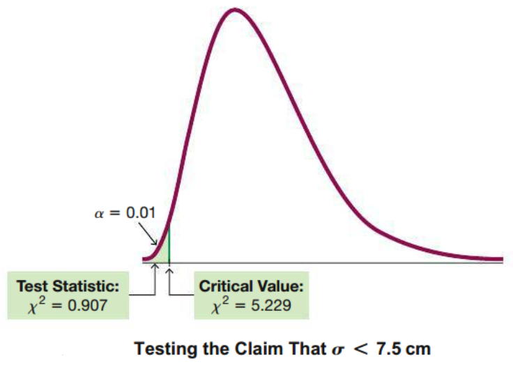
From \(\chi^2\) table,
\[ \text {The critical value of } \chi^2 = 5.229 \text { at } \alpha = 0.01. \\ \] Hence, we reject \(H_0\).
Confidence Interval Calculation:
\[ \sqrt{ \dfrac{(n-1)s^2}{\chi_R^2} } < \sigma < \sqrt{ \dfrac{(n-1)s^2}{\chi_L^2} } \\ \sqrt{ \dfrac{(16-1)3.4}{30.578} } < \sigma < \sqrt{ \dfrac{(16-1)3.4}{5.229} } \\ 1.3 \text{ cm } < \sigma < 3.1 \text { cm } \]